 Travis Horn
Building an Enrollment Prediction System with Machine Learning

Schools need accurate enrollment forecasting for stability and success. Forecasting informs decisions they face annually: staffing, resource allocation, and budget planning. When projections are accurate, schools can hire the exact number of teachers needed to maintain good student-teacher ratios, ensuring that no classroom is overcrowded and no teacher is overburdened. Enrollment also dictates the number of desks and devices to purchase, the logistics of bus routes, and more. Accurate predictions prevent budget shortfalls or wasted surplus. Every dollar can be directed toward enhancing a student’s education.
Traditional approaches often rely on manual spreadsheets, static formulas, simple cohort survival ratios, and rigid rolling averages. These methods are reactive and prone to human error. They don’t account for complex, non-linear variables, such as shifting local demographics and enrollment volatility. Administrators are left with basic arithmetic and “gut feeling.” We want to avoid last-minute hiring and empty classrooms that drain resources.
I want to treat enrollment forecasting as a data science problem. Join me as I document how I built a machine learning enrollment prediction system using Python. It is a pipeline designed to ingest historical data and intelligently predicts enrollment for the next future year. This system uses ML libraries like Scikit-Learn to train and evaluate multiple models, and automatically handles the heavy lifting of data cleaning, feature engineering, and hyperparameter tuning. I built a reliable system that analyzes trends and gives me data-backed confidence in the numbers it generates.
To find the right tool for the job, I set up a competition between three approaches: a standard Linear Regression baseline, a Gradient Boosting Regressor, and a Random Forest Regressor.
Data: The Foundation of Predictions
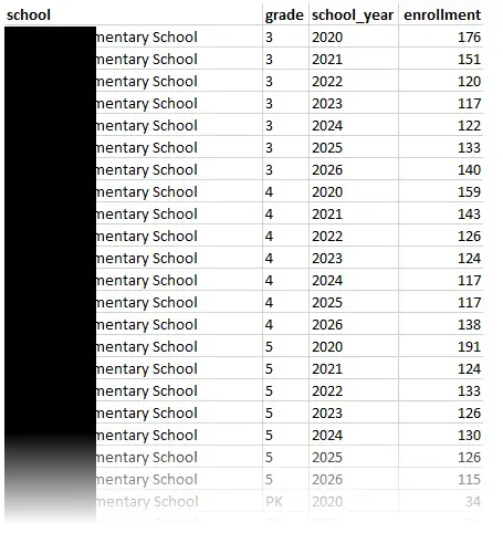
Data fuels this engine. For the pipeline to function, I needed a well-defined
input format. I chose a clean, flat CSV file with four essential columns:
school, grade, school_year, and enrollment. This granularity is
non-negotiable. It allows the model to distinguish between, say, a growing
kindergarten class at a specific elementary school and a shrinking senior class
at a high school. Since this input format is well-defined, I could more easily
build feature engineering scripts to generate the lag, rolling average, and
other features necessary for training.
To generate a CSV file in this format, I wrote a SQL query tailored for the specific information system that contained my source data. Consistency is key in time-series forecasting, so I implemented a “Count Date” methodology, capturing enrollment numbers specifically on a particular day of the year for each academic year. This ensures we aren’t comparing, say, a September roster from 2018 with a January roster from 2023. The query also normalized internal grade level codes.
I wrote the query and executed it on the information system to output the data needed to generate predictions.
This query is just an example, but demonstrates the concept:
SELECT
    s.name AS school,
    -- Grade normalization
    CASE
        WHEN e.grade_level_code IN ('P1', 'P2', 'PK_AM', 'PK_PM') THEN 'PK'
        WHEN e.grade_level_code IN ('KG', 'K_FULL', '00') THEN 'K'
        ELSE e.grade_level_code -- Keeps 1-12 as is, assuming they are standard
    END AS grade,
    e.school_year,
    COUNT(DISTINCT e.student_id) AS enrollment
FROM enrollment e
JOIN schools s ON e.school_id = s.id
WHERE
    -- Count date methodology
    CAST(CONCAT(e.school_year, '-10-01') AS DATE)
        BETWEEN e.entry_date AND COALESCE(e.exit_date, '9999-12-31')
GROUP BY
    s.name,
    2, -- Refers to the calculated 'grade' column (the CASE statement)
    e.school_year
Initial Exploration
Before writing any training code, I wrote some exploration code to output some charts and graphs to help me visualize the historical data to understand the baseline volatility I was dealing with.
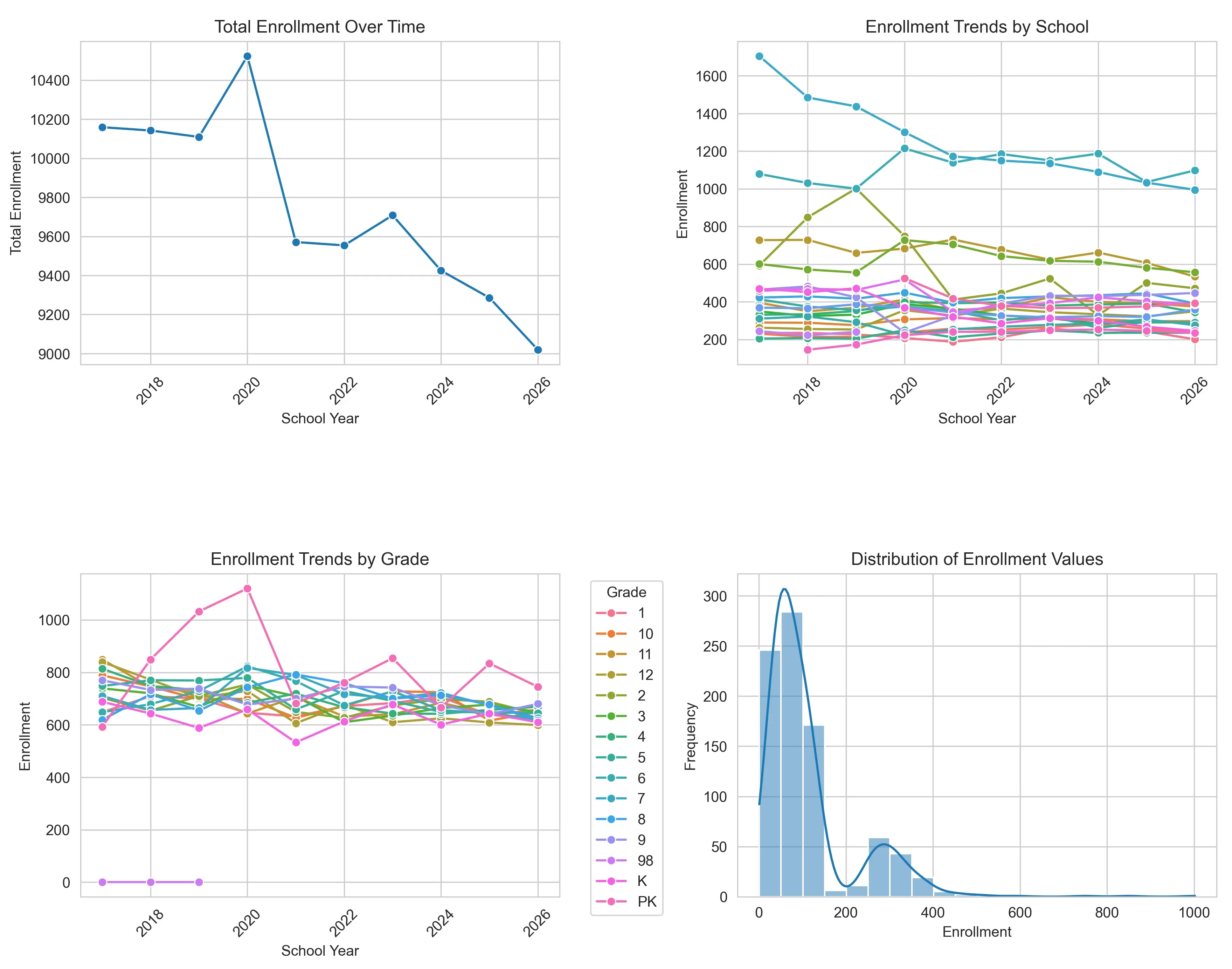
The numbers are definitely not static. There is a significant peak around 2020, reaching nearly 10,500 students, followed by a drop the very next year. This volatility is most likely due to the COVID-19 pandemic. Since that reset, the data shows a brief recovery followed by a steady downward trajectory through 2026. This proves that a simple “average growth” formula would not suffice. The data is a complex, non-linear narrative that requires a model capable of adapting to sudden shifts.
Digging deeper into the dataset via box plots exposes more variance hidden within the aggregate numbers.
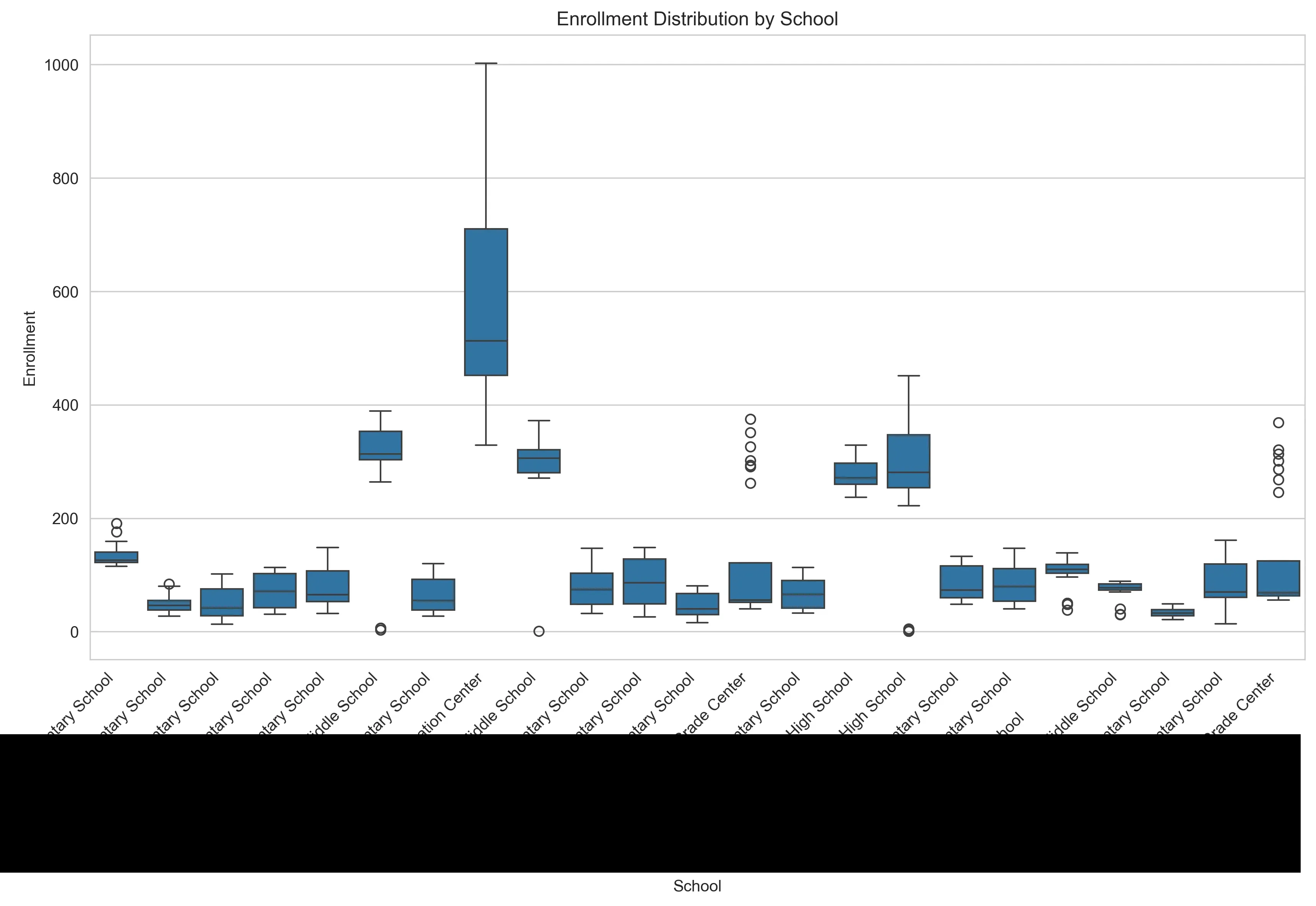
The school-level distribution reveals big size differences. Some schools operate with vastly larger enrollment than others. In this dataset, the word “average” is not very meaningful.
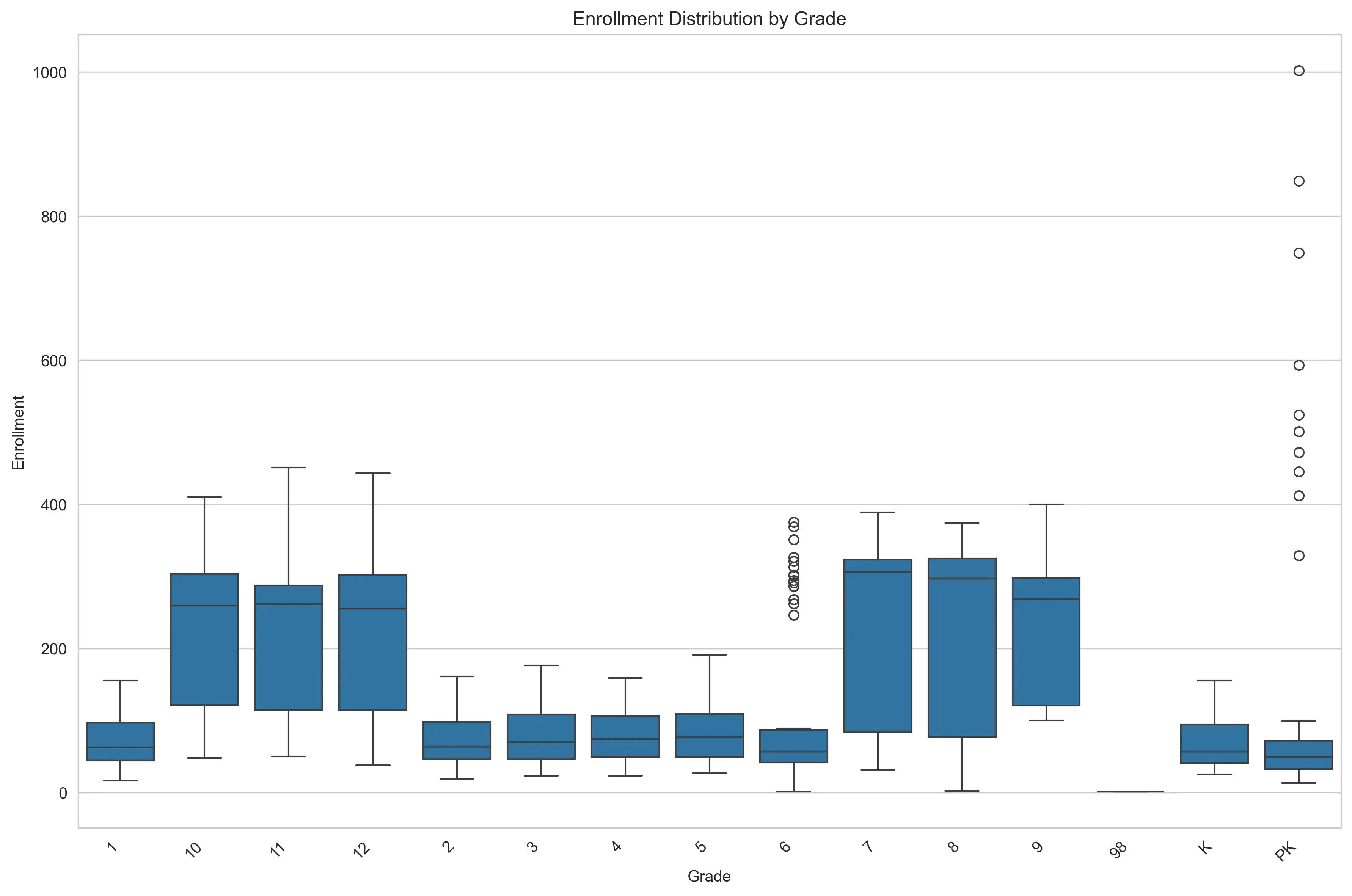
Similarly, the grade-level breakdown highlights more patterns. High school cohorts (grades 9-12) display significantly higher counts and wider volatility compared to the relatively stable elementary years. This means that “School” and “Grade” have to be treated as categorical features. A model trained on general trends without these specific contexts would fail to capture the uniqueness of each building.
The Prediction Pipeline
With exploration done, I built the main pipeline script. It acts as the
orchestrator of the project. It imports the data cleaning, feature generation,
model training, and evaluation scripts into one easy-to-use command line tool.
Using Python’s argparse library, it allows me to interact with the system from
the terminal, accepting arguments for the specific prediction year or a
preferred training window. Under the hood, the script executes a sequential
workflow: it first ingests the raw data to build the features, then initiates
the training tournament to identify the best performing algorithm (usually the
Random Forest), and finally applies that champion model to generate and save the
future enrollment forecasts to a CSV file. The goal is to make this multi-step
data science experiment more deployable.
Again, this code is just a demonstration of the concept:
import argparse
import sys
import feature_engineering as fe # Handles data cleaning and feature generation
import model_training as mt # Handles the algorithm tournament
import forecasting as fc # Handles applying the model to future dates
def main():
# Setup arguments
parser = argparse.ArgumentParser()
parser.add_argument(
'--target_year',
type=int,
required=True
)
parser.add_argument(
'--window',
type=int,
default=5
)
args = parser.parse_args()
try:
# Ingestion and feature engineering
training_data = fe.create_dataset(lookback_window=args.window)
# Model training competition
champion_model = mt.find_best_model(training_data)
# Forecasting
forecast_df = fc.predict_future(champion_model, year=args.target_year)
# Output
output_filename = f"forecast_{args.target_year}.csv"
forecast_df.to_csv(output_filename, index=False)
except Exception as e:
print(f"\nError: The pipeline failed.\n{e}")
sys.exit(1)
if __name__ == "__main__":
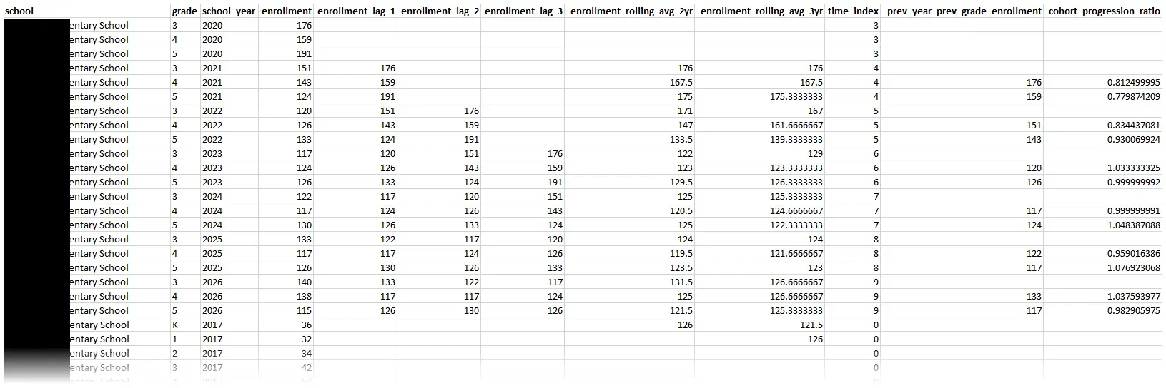
main()The main pipeline script imports the more focused, individual scripts, such as the feature engineering script. Feature engineering provides the context the model needs to learn. In the feature engineering script, I transform the flat CSV into a richer training set. The script starts with enforcing logical sort orders for grades (ensuring ‘Kindergarten’ comes before ‘1st Grade’) and filtering out anomalies. From there, it constructs temporal features, generating lag variables and rolling averages that allow the model to see recent history at a glance. Most importantly, I implemented a custom function to create cohort features. These features simulate the natural flow of a school system. By mapping the “previous grade” from the “previous year” to the current row, I calculate a cohort progression ratio. This critical feature teaches the model that the size of this year’s 3rd-grade class is the strongest predictor for next year’s 4th-grade class, effectively capturing the “survival rate” of cohorts as they move through the district.
Here’s the basic concept:
import pandas as pd
import numpy as np
def create_dataset(lookback_window=5):
df = pd.read_csv('raw_enrollment_data.csv')
# Enforce grade sort order
grade_map = {'PK': -1, 'K': 0, '1': 1, '2': 2, '3': 3, '4': 4,
'5': 5, '6': 6, '7': 7, '8': 8, '9': 9, '10': 10, '11': 11, '12': 12}
df['grade_id'] = df['grade'].map(grade_map)
df = df.sort_values(by=['school', 'grade_id', 'school_year'])
# Temporal features
grouper = df.groupby(['school', 'grade'])
df['enrollment_lag_1'] = grouper['enrollment'].shift(1)
df['enrollment_lag_2'] = grouper['enrollment'].shift(2)
df['enrollment_lag_3'] = grouper['enrollment'].shift(3)
# Rolling averages smooth out noisy years
df['enrollment_rolling_avg_2yr'] = grouper['enrollment'].transform(lambda x: x.rolling(2).mean())
df['enrollment_rolling_avg_3yr'] = grouper['enrollment'].transform(lambda x: x.rolling(3).mean())
# Simple numeric time index for regression models (e.g., 2018 -> 0, 2019 -> 1)
df['time_index'] = df['school_year'] - df['school_year'].min()
# Cohort features
df['target_prev_grade_id'] = df['grade_id'] - 1
df['target_prev_year'] = df['school_year'] - 1
lookup_df = df[['school', 'grade_id', 'school_year', 'enrollment']].copy()
lookup_df.rename(columns={'enrollment': 'prev_year_prev_grade_enrollment'}, inplace=True)
df = pd.merge(
df,
lookup_df,
left_on=['school', 'target_prev_grade_id', 'target_prev_year'],
right_on=['school', 'grade_id', 'school_year'],
how='left',
suffixes=('', '_lookup')
)
# Progression ratio
df['cohort_progression_ratio'] = df['enrollment'] / df['prev_year_prev_grade_enrollment']
df['cohort_progression_ratio'] = df['cohort_progression_ratio'].fillna(1.0)
# Cleanup and export
final_cols = [
'school', 'grade', 'school_year',
'enrollment_lag_1', 'enrollment_lag_2', 'enrollment_lag_3',
'enrollment_rolling_avg_2yr', 'enrollment_rolling_avg_3yr',
'time_index', 'prev_year_prev_grade_enrollment', 'cohort_progression_ratio'
]
# Remove rows with NaN created by lags (the first few years of data)
clean_df = df.dropna(subset=['enrollment_lag_3'])[final_cols]
return clean_df
if __name__ == "__main__":
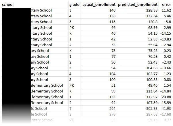
create_dataset()And a sample of the output:
With the features ready, I needed a way to determine how accurate the models were. I implemented a training strategy split across a couple files. First, I used one file to establish a sanity check using a simple Linear Regression baseline. If my advanced models couldn’t beat this, I was over-engineering. Linear regression basically draws a trend line through the historic data points and then extends that line out into the future to see where enrollment will be in the future.
import pandas as pd
from sklearn.linear_model import LinearRegression
from sklearn.metrics import mean_absolute_error

def run_baseline(df):
    # Time-based split
    test_year = df['school_year'].max()

    train_df = df[df['school_year'] < test_year]
    test_df  = df[df['school_year'] == test_year]

    # Define features
    features = [
        'enrollment_lag_1',
        'enrollment_lag_2',
        'enrollment_rolling_avg_2yr',
        'time_index',
        'cohort_progression_ratio'
    ]
    target = 'enrollment'

    X_train = train_df[features]
    y_train = train_df[target]

    X_test  = test_df[features]
    y_test  = test_df[target]

    # Train
    model = LinearRegression()
    model.fit(X_train, y_train)

    # Evaluation
    predictions = model.predict(X_test)
    mae = mean_absolute_error(y_test, predictions)

    return model, mae
Then I built more advanced models in a separate file: Random Forest and Gradient Boosting Regressors. These models are generally excellent at handling non-linear relationships. To test accuracy, I simulated a real-world scenario by training on all historical data except the most recent year, then asked the models to “predict” that known final year (e.g., train on 2016-2024, test on 2025). This “out-of-time” validation provides the feedback loop needed to pick a winning model.
import pandas as pd
from sklearn.ensemble import RandomForestRegressor, GradientBoostingRegressor
from sklearn.metrics import mean_absolute_error

def find_best_model(df):
    # Time-based split
    test_year = df['school_year'].max()
    train_df = df[df['school_year'] < test_year]
    test_df  = df[df['school_year'] == test_year]

    # Define features
    features = [
        'enrollment_lag_1', 'enrollment_lag_2',
        'enrollment_rolling_avg_2yr', 'time_index',
        'cohort_progression_ratio'
    ]
    target = 'enrollment'

    X_train = train_df[features]
    y_train = train_df[target]
    X_test  = test_df[features]
    y_test  = test_df[target]

    # Contestants
    models = {
        "Random Forest": RandomForestRegressor(n_estimators=100, random_state=42),
        "Gradient Boosting": GradientBoostingRegressor(n_estimators=100, random_state=42)
    }

    # Competition
    best_mae = float('inf') # Start with infinite error
    champion = None

    for name, model in models.items():
        # Train
        model.fit(X_train, y_train)

        # Predict
        predictions = model.predict(X_test)

        # Evaluate
        mae = mean_absolute_error(y_test, predictions)

        # Determine winner
        if mae < best_mae:
            best_mae = mae
            champion = model

    # Retrain the champion on ALL data (Train + Test) before forecasting the future.
    champion.fit(df[features], df[target])

    return champion
While the default settings in Scikit-Learn are a solid starting point, I wanted to squeeze every ounce of accuracy out of the system. I wrote a script to automate the process of tuning the model’s hyperparameters. I started by targeting the Random Forest’s architecture. Instead of testing every possible combination of parameters (which takes forever), I implemented RandomizedSearchCV. This technique samples a wide range of possibilities for parameters like the number of trees (n_estimators), maximum depth (max_depth), etc. The script identifies the specific configuration that produces the best predictions.
import pandas as pd
import numpy as np
from sklearn.ensemble import RandomForestRegressor
from sklearn.model_selection import RandomizedSearchCV

def optimize_random_forest(df):
    # Prepare data
    features = [
        'enrollment_lag_1', 'enrollment_lag_2',
        'enrollment_rolling_avg_2yr', 'time_index',
        'cohort_progression_ratio'
    ]
    target = 'enrollment'

    X = df[features]
    y = df[target]

    # Define the parameter grid
    param_grid = {
        # How many trees to build (More is usually better but slower)
        'n_estimators': [100, 200, 300, 500],
        # How complex can each tree get (Too deep = overfitting)
        'max_depth': [None, 10, 20, 30],
        #  Minimum students required to create a new logic branch
        'min_samples_split': [2, 5, 10]
    }

    # Initialize base model
    rf = RandomForestRegressor(random_state=42)

    # Randomized search
    search = RandomizedSearchCV(
        estimator=rf,
        param_distributions=param_grid,
        n_iter=10,
        cv=3,            # Cross-Validation: Splits data 3 ways to verify results
        verbose=1,
        n_jobs=-1,       # Use all computer processors
        random_state=42
    )

    search.fit(X, y)

    # Results
    best_params = search.best_params_
    best_score = search.best_score_ # R-squared value

    # Return the optimized model ready for use
    return search.best_estimator_
To be able to import these files into the main pipeline, we’ll need a model_training file that glues everything together:
import baseline_model
import advanced_models
import tuning

def find_best_model(df):
    baseline_model.run_baseline(df)
    champion = advanced_models.find_best_model(df)
    if champion.name == "Random Forest":
        champion = tuning.optimize_random_forest(df)

    features = [
        'enrollment_lag_1', 'enrollment_lag_2',
        'enrollment_rolling_avg_2yr', 'time_index',
        'cohort_progression_ratio'
    ]

    champion.fit(df[features], df['enrollment'])

    return champion
Choosing the Best Model
When we crunch the numbers, the distinction between the models is a landslide.
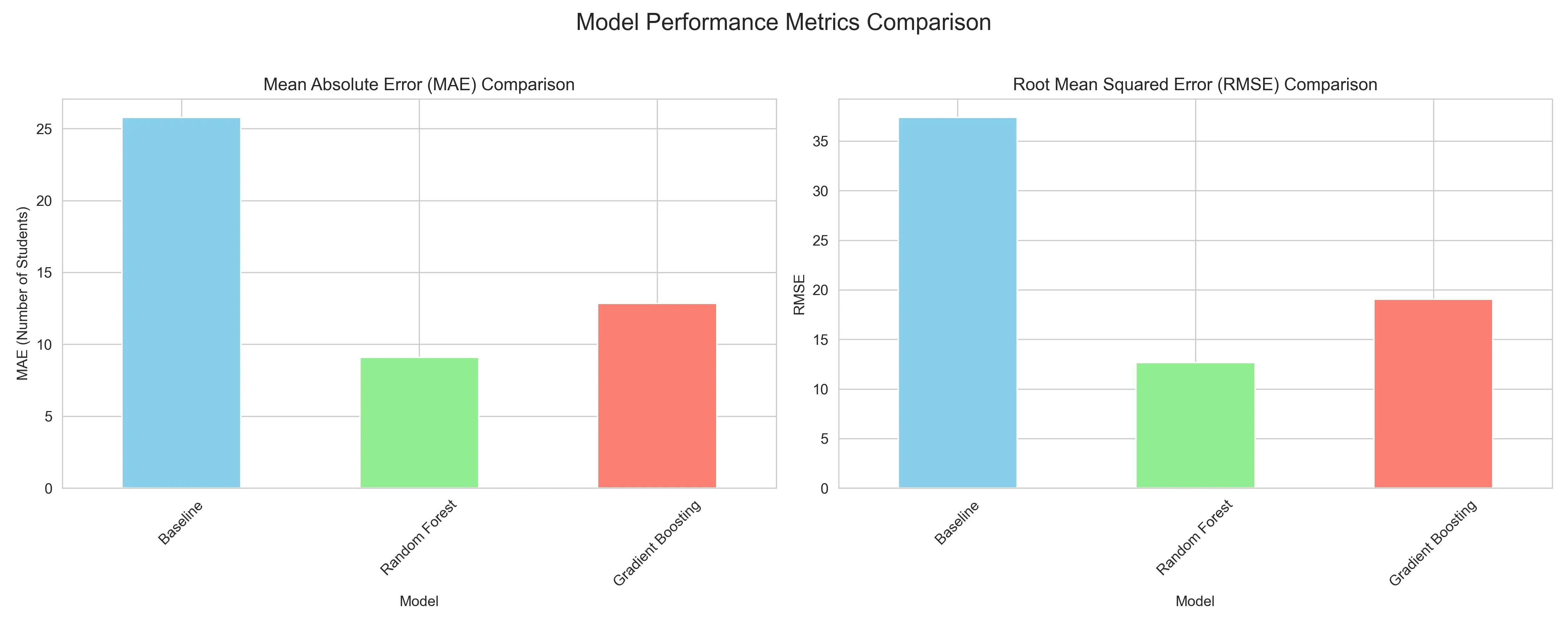
The baseline Linear Regression yields a Mean Absolute Error (MAE) of 25.78, missing the mark by an entire classroom of students on average. The Gradient Boosting model offers a respectable improvement (MAE 12.84). But the Random Forest Regressor proves to be the best, driving the error down to only 9.1 students per prediction. A Root Mean Squared Error (RMSE) of 12.67 further confirms its stability. The RMSE result indicates that it isn’t just accurate on average, but also less prone to wild outliers.
Let’s see where the models were succeeding or failing.
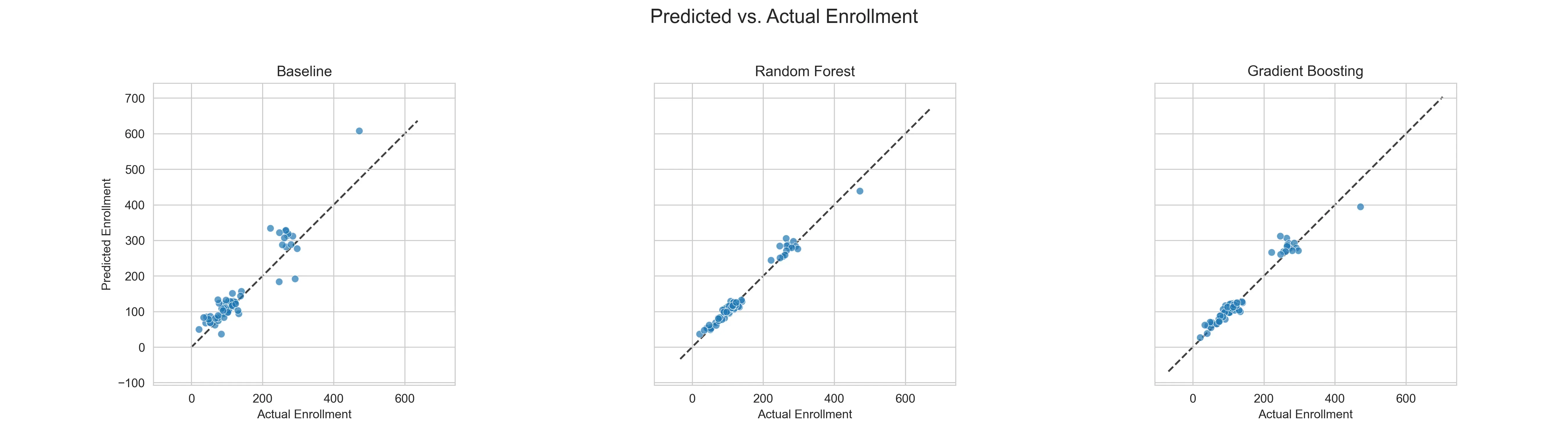
While the baseline’s predictions scatter loosely, guessing with a wide margin of error, the Random Forest’s predictions hug the diagonal “perfect fit” line.
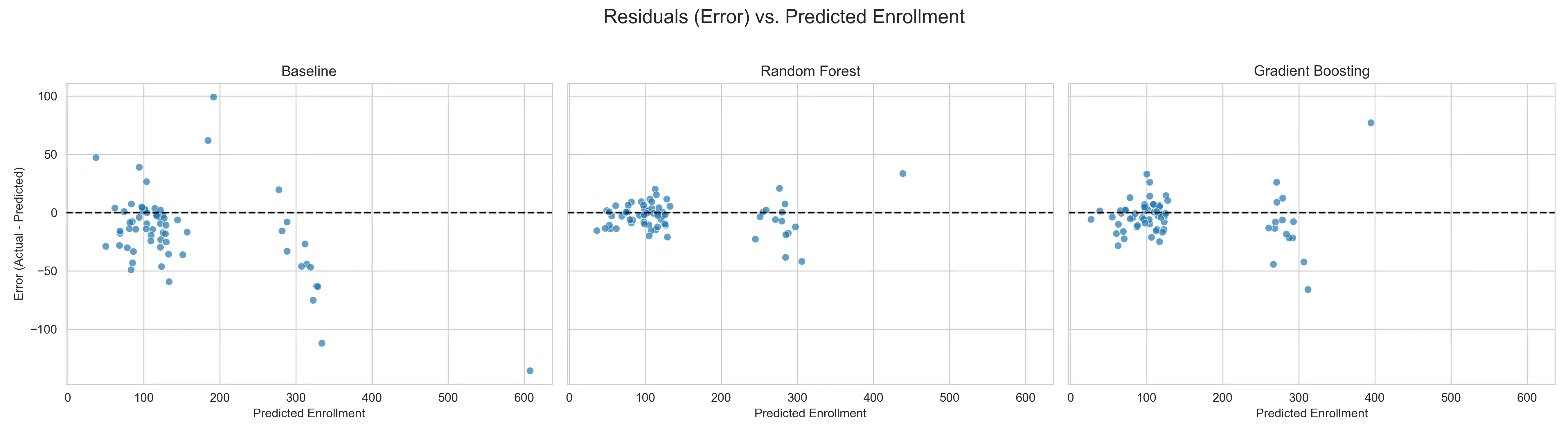
Even more telling is the residual analysis, which plots the error for every single prediction. In a healthy model, these errors should look like random noise centered around zero. The Baseline fails, showing a bias where errors grow significantly larger as enrollment numbers increase. The Random Forest’s residuals, however, remain tightly clustered around the zero line across the board. It’s pretty good across all school sizes and grade levels.
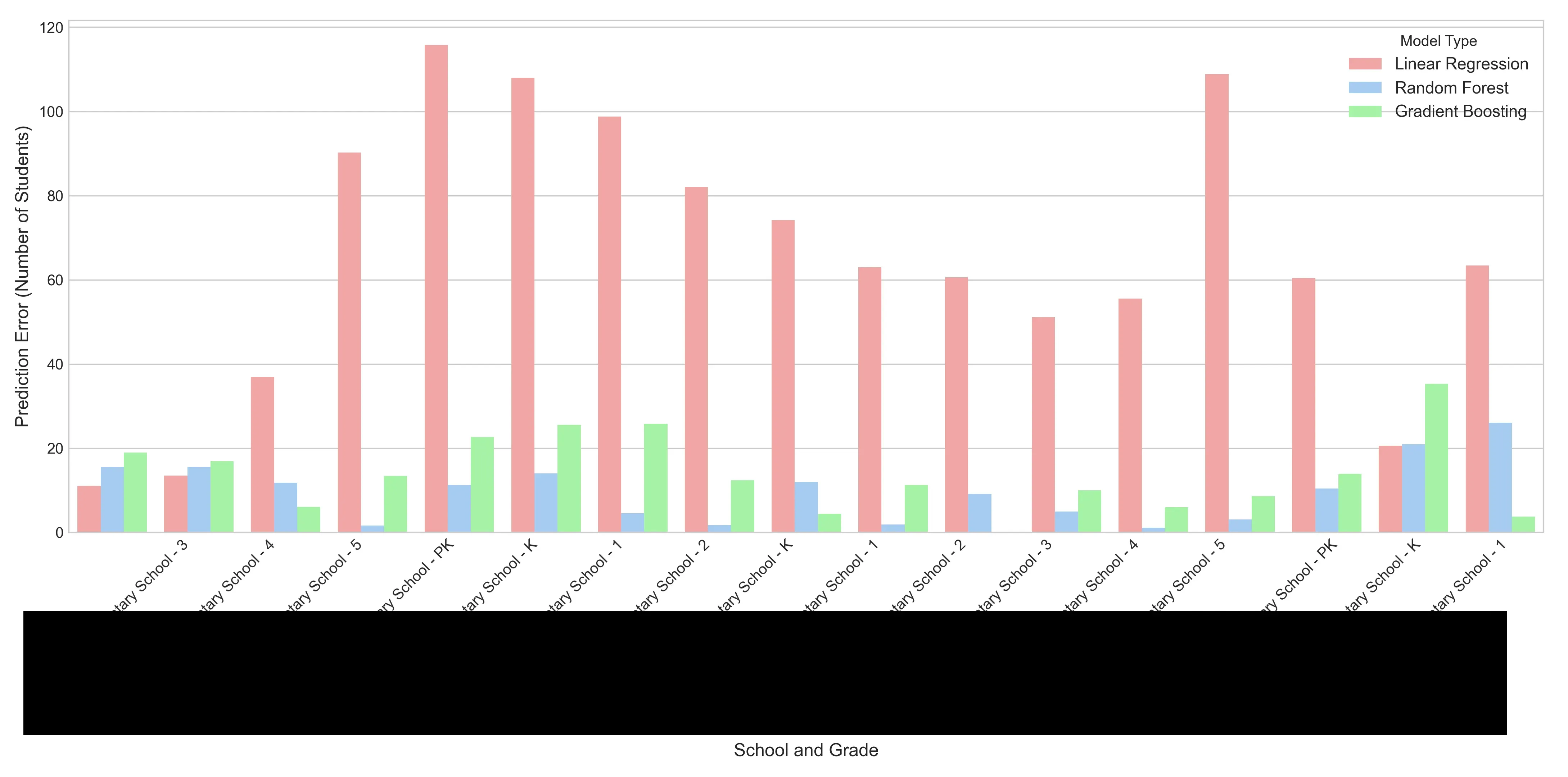
We can also look at this from a “crystal ball” analysis perspective. This visualization useful to non-technical users who need to understand the performance of the models. For each school and grade combination, the chart shows how many students the model was off. You can see that the baseline linear regression model is almost always off by the most amount of students and the random forest model is off by the least.
The Random Forest Regressor demonstrated the most robust understanding of the underlying data dynamics. Enrollment forecasting is a complex interaction of cohort survival rates, varying school capacities, and demographic shifts. Linear Regression isn’t flexible enough and Gradient Boosting struggles with consistency for this type of data. But the Random Forest excels here. By averaging the predictions of hundreds of decision trees, it cancels out individual errors and overfitting. This makes the Random Forest forecast precise enough for staffing and stable enough for budgeting.
The Training Window Experiment
I also questioned how usable the pre-2020 data was, given how drastically the pandemic altered everything. To test this recency bias hypothesis, I wrote a script that retrained the Random Forest on restricted windows (3, 5, and 7 years) to see if a shorter memory improved accuracy.
import pandas as pd
from sklearn.ensemble import RandomForestRegressor
from sklearn.metrics import mean_absolute_error

def test_window_sensitivity(df):
    # We test on the most recent known year
    test_year = df['school_year'].max()

    # Compare these specific history lengths
    windows = [3, 5, 7]

    features = [
        'enrollment_lag_1', 'enrollment_lag_2',
        'enrollment_rolling_avg_2yr', 'time_index',
        'cohort_progression_ratio'
    ]
    target = 'enrollment'

    for lookback in windows:
        # Filter
        start_year = test_year - lookback
        subset_df = df[df['school_year'] >= start_year].copy()

        # Split
        train_df = subset_df[subset_df['school_year'] < test_year]
        test_df  = subset_df[subset_df['school_year'] == test_year]

        # Train and evaluate
        model = RandomForestRegressor(n_estimators=100, random_state=42)
        model.fit(train_df[features], train_df[target])

        predictions = model.predict(test_df[features])
        error = mean_absolute_error(test_df[target], predictions)

        print(f"{lookback}-year window MAE: {error:.2f}")
The model actually performed worse when restricted to recent history, with the 3-year window spiking the error rate (RMSE 16.00) compared to the baseline full history (RMSE 12.67). It turns out that even “outdated” pre-pandemic data provides valuable variance that helps the Random Forest distinguish between genuine trends and temporary blips. For this specific dataset, maximizing the historical context yields the best results.
Outputs and Interpretations
The ultimate deliverable of this project isn’t the model itself, but the predictions it generates. I designed the output CSV to be immediately consumable by non-technical users, mirroring the format of the input data but swapping historical data for future forecasts.
import pandas as pd
import numpy as np

def predict_future(model, year):
    # Identify most recent data
    df = pd.read_csv('raw_enrollment_data.csv')
    latest_known_year = df['school_year'].max()

    # Filter for the current active students
    current_roster = df[df['school_year'] == latest_known_year].copy()

    # Construct future dataframe
    future_df = current_roster[['school', 'grade']].copy()
    future_df['school_year'] = year

    # Generate features

    future_df['enrollment_lag_1'] = current_roster['enrollment'].values

    # For this simplified demo, we assume stability for older lags/ratios.
    # In a real production system, you would calculate these recursively.
    future_df['enrollment_lag_2'] = current_roster['enrollment'].values
    future_df['enrollment_rolling_avg_2yr'] = current_roster['enrollment'].values
    future_df['cohort_progression_ratio'] = 1.0  # Assumes 100% survival rate for the demo

    # Update the time index (e.g., if last year was index 5, this is index 6)
    future_df['time_index'] = 100 # Arbitrary high number for the future

    # Predict
    features = [
        'enrollment_lag_1', 'enrollment_lag_2',
        'enrollment_rolling_avg_2yr', 'time_index',
        'cohort_progression_ratio'
    ]

    predictions = model.predict(future_df[features])

    # Format output
    future_df['enrollment_prediction'] = np.round(predictions).astype(int)
    final_output = future_df[['school', 'grade', 'school_year', 'enrollment_prediction']]

    return final_output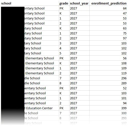
It provides a granular, row-by-row breakdown that tells us, for example, that a particular elementary school should prepare for exactly 103 third-graders in 2027 while another elementary school needs to staff for a Pre-K cohort of 64. This standardized format ensures that the data can be opened in Excel for manual review or imported into dashboard tools for more visualization.
In addition to the predictions, I was also able to output many files detailing my evaluation along the way. Transparency is just as important as accuracy, so I ensured the pipeline leaves a detailed paper trail. This includes the visuals you see on this post, and also granular CSV reports on each model’s performance and comparisons between them.
This comprehensive documentation helps demystify some of the “black box” problems that come with machine learning. It can provide proof to justify the numbers.
Conclusion
Building this system has transformed a guessing game into a science. By engineering features and benchmarking different algorithms, I created a machine learning model that achieves an MAE of 9.1 and an RMSE of 12.67. I can now provide the foundation for a proactive strategy, where decisions on allocating resources are backed by statistical evidence rather than historical inertia.
Machine learning models require continuous refinement. The next phase of development will focus on more data ingestion. How about external indicators like housing permits and birth rates? These could capture other shifts even before a student sets foot in a classroom. On the engineering side, I aim to build a direct connection to the information system, allowing for real-time model retraining and automated drift detection. I also plan to integrate this system with existing dashboards to further empower non-technical users.
Cover photo by Pawel Czerwinski on Unsplash.